library(here)
library(tidyverse)
library(knitr)
library(stargazer)
library(plm)
library(pglm)
library(dplyr)
library(MatchIt)
library(lmtest)
library(RItools)
library(sandwich)
library(estimatr)
library(Hmisc)Did Smoking Mothers Have Lowered Weight Children?
Causal Inference
R
Summary and Conclusion
The analysis aimed to estimate the causal effect of maternal smoking during pregnancy on infant birth weight. Initial comparisons showed a significant difference in birth weights between infants of smoking and non-smoking mothers. However, confounding variables suggested that the groups were not comparable.
Propensity score matching was applied to address these confounders. Post-matching tests indicated successful balancing of the treatment and control groups. The final analysis showed that maternal smoking causally reduces infant birth weight by an average of 13 grams, after accounting for confounding variables. This result highlights the importance of proper matching techniques in observational studies to draw valid causal inferences
Project Begins:
The goal is to estimate the causal effect of maternal smoking during pregnancy on infant birth weight using the treatment ignorability assumptions. The data are taken from the National Natality Detail Files, and the extract “SMOKING_EDS241.csv”’ is a random sample of all births in Pennsylvania during 1989-1991. Each observation is a mother-infant pair. The key variables are:
The outcome and treatment variables are:
birthwgt=birth weight of infant in grams
tobacco=indicator for maternal smoking
The control variables are:
mage (mother’s age), meduc (mother’s education), mblack (=1 if mother identifies as Black), alcohol (=1 if consumed alcohol during pregnancy), first (=1 if first child), diabete (=1 if mother diabetic), anemia (=1 if mother anemic)
# Load data
smoking_data <- read_csv(here("featured_projects/econometrics/data/SMOKING_EDS241.csv"))
Mean Differences, Assumptions, and Covariates
For conducting t-test, it is important to have population divided into treatment and control group. Since this experiment already has that information, I can segregate them into two tables and perform t-tests.
## calculating difference using t.test when tobacco is 1 and 0
smoking_mothers = smoking_data %>% filter(tobacco == 1)
non_smoking_mothers = smoking_data %>% filter(tobacco == 0)

#peform t-test to see if the difference is significant in other covariates
t.test(smoking_mothers$birthwgt, non_smoking_mothers$birthwgt)
    Welch Two Sample t-test

data:  smoking_mothers$birthwgt and non_smoking_mothers$birthwgt
t = -58.932, df = 26945, p-value < 2.2e-16
alternative hypothesis: true difference in means is not equal to 0
95 percent confidence interval:
 -252.6727 -236.4060
sample estimates:
mean of x mean of y
 3185.747  3430.286
The mean difference is 244.539 grams between children from smoker and non-smoker mothers, which is significant at 5%. The assumptions for this mean difference to hold are ignorability (no other confounding variables influencing the outcome) and common support (there is sufficient overlap between the treatment and control group). If these assumptions are satisfied, I can infer the difference is actually due to smoking and not due to random chance.
I can test those assumptions with t-tests for numeric covariates, and proportion test for categorical covariates The following code achives that:
#set options to have maximum 5 decimal
options(digits=5)
## For continuous variables I can use the t-test
#t.test()
education <- t.test(smoking_mothers$meduc, non_smoking_mothers$meduc)
age <- t.test(smoking_mothers$mage, non_smoking_mothers$mage)
birthwht <- t.test(smoking_mothers$birthwgt, non_smoking_mothers$birthwgt)

## For binary variables I should use the proportions test
#prop.test()
alcohol <- prop.test(table(smoking_mothers$alcohol), table(non_smoking_mothers$alcohol))
first_child <-prop.test(table(smoking_mothers$first), table(non_smoking_mothers$first))
diabetes<- prop.test(table(smoking_mothers$diabete), table(non_smoking_mothers$diabete))
anaemia <- prop.test(table(smoking_mothers$anemia),  table(non_smoking_mothers$anemia))
black   <- prop.test(table(smoking_mothers$mblack),  table(non_smoking_mothers$mblack))

#-------------- Covariate Calculations and Tables

# create dataframe of coefficents from above results including
# first column should be variable name, then mean of estimate for sample 1, then
# mean of sample 2, then p values
table <- data.frame(
  variable = c("birthweight", "education", "age", "alcohol", "first_child", "diabetes", "anaemia", "black"),
  smoking_mothers = c(birthwht$estimate[1], education$estimate[1], age$estimate[1],
                      sum(smoking_mothers$alcohol)/length(smoking_mothers$alcohol),
                      sum(smoking_mothers$first)/length(smoking_mothers$first),
                      sum(smoking_mothers$diabete)/length(smoking_mothers$diabete),
                      sum(smoking_mothers$anemia)/length(smoking_mothers$anemia),
                      sum(smoking_mothers$mblack)/length(smoking_mothers$mblack)),

  non_smoking_mothers = c(birthwht$estimate[2], education$estimate[2], age$estimate[2],
                          sum(non_smoking_mothers$alcohol)/length(non_smoking_mothers$alcohol),
                          sum(non_smoking_mothers$first)/length(non_smoking_mothers$first),
                          sum(non_smoking_mothers$diabete)/length(non_smoking_mothers$diabete),
                          sum(non_smoking_mothers$anemia)/length(non_smoking_mothers$anemia),
                          sum(non_smoking_mothers$mblack)/length(non_smoking_mothers$mblack)),

  p_value = round(c(birthwht$p.value,
                    education$p.value,
                    age$p.value,
                    alcohol$p.value,
                    first_child$p.value,
                    diabetes$p.value,
                    anaemia$p.value,
                    black$p.value), 6))

print(table)
variable smoking_mothers non_smoking_mothers p_value
1 birthweight 3.1857e+03 3.4303e+03 0
2 education 1.1921e+01 1.3239e+01 0
3 age 2.5539e+01 2.7453e+01 0
4 alcohol 4.4182e-02 7.1033e-03 0
5 first_child 3.6459e-01 4.3609e-01 0
6 diabetes 1.7519e-02 1.7364e-02 0
7 anaemia 1.4103e-02 7.8005e-03 0
8 black 1.3541e-01 1.0863e-01 0Interpretation: The result shows that the population sample on treated and control group is dissimilar. The p values are less than .05, which means alternative hypothesis shoule be accepted. Alternative hypothesis for this test is: there is difference between treated and control group.
So far, I know there is already a difference in the two samples. But we can still quantify how much these covariates influence these biased samples. The following chunk will do that by calculating average treatment effects with a regression model for these biased groups.
# ATE Regression univariate
tobacco_univariate <- lm(birthwgt ~ tobacco, data = smoking_data)

# ATE with covariates
tobacco_covariates <- lm(birthwgt ~  tobacco + mage +  meduc +
                           mblack + alcohol + first + diabete + anemia,
                      data = smoking_data)

## create combined table
stargazer(tobacco_univariate, tobacco_covariates, type = "text",
          out.header = TRUE,
          title = "Regression with and without controls",
          notes.label = "significance level")
Regression with and without controls
===========================================================================
                                      Dependent variable:
                    -------------------------------------------------------
                                           birthwgt
                                (1)                         (2)
---------------------------------------------------------------------------
tobacco                     -244.540***                 -228.070***
                              (4.079)                     (4.177)

mage                                                      -0.694*
                                                          (0.357)

meduc                                                    11.688***
                                                          (0.860)

mblack                                                  -240.030***
                                                          (5.106)

alcohol                                                  -77.350***
                                                          (13.465)

first                                                    -96.944***
                                                          (3.447)

diabete                                                  73.228***
                                                          (12.104)

anemia                                                     -4.796
                                                          (16.754)

Constant                    3,430.300***                3,362.300***
                              (1.791)                     (11.927)

---------------------------------------------------------------------------
Observations                   94,173                      94,173
R2                             0.037                       0.072
Adjusted R2                    0.037                       0.072
Residual Std. Error     493.750 (df = 94171)        484.730 (df = 94164)
F Statistic         3,594.300*** (df = 1; 94171) 909.180*** (df = 8; 94164)
===========================================================================
significance level                              *p<0.1; **p<0.05; ***p<0.01
If I have to see the result above, seems like all covariates are responsible for change in birthweights in the smoking and non smoking mothers. But since the treated and control groups are dissimilar, it should not be inferred that these covariates are producing change.
I can do one more test before I process the data to make them true. I can test if any of the covariates have a similar population between the treated and control groups already. I can use chi-squared tests among all these variables to see which one truly represents a similar population being compared.
# perform balance test
x <- xBalance(tobacco ~ mage +  meduc + mblack + alcohol + first + diabete + anemia + birthwgt,  data = smoking_data,
         report=c("std.diffs","chisquare.test", "p.values"))

#use staragazer to present the results
as.data.frame(x[1]) %>%
   #round last column to 5 digit
  mutate_if(is.numeric, round, 5) %>%
  #rename columns based on number index
  setNames(c( "chi-Square/standard difference test", "p-value"))
chi-Square/standard difference test p-value
mage -0.36194 0.0000
meduc -0.64374 0.0000
mblack 0.08439 0.0000
alcohol 0.31525 0.0000
first -0.14500 0.0000
diabete 0.00119 0.8858
anemia 0.06670 0.0000
birthwgt -0.49527 0.0000Only the diabetic covariate is similar between sample group at this point. What this means is that the population samples between treatment and control group are similar only in regards to diabetes.
Lets also calculate propensity estimation for this biased sample:
Propensity Score Estimation for the biased Treated and control Groups
## Propensity Scores estimation with logistic regression
mother_prospensityscore <- glm(tobacco ~  mage +  meduc +
                           mblack + alcohol + first + diabete + anemia + birthwgt, data = smoking_data,
                              family = binomial())

## create a table of coefficients
stargazer:: stargazer(mother_prospensityscore, type = "text")
=============================================
                      Dependent variable:
                  ---------------------------
                            tobacco
---------------------------------------------
mage                       -0.040***
                            (0.002)

meduc                      -0.288***
                            (0.005)

mblack                     -0.361***
                            (0.028)

alcohol                    1.962***
                            (0.062)

first                      -0.460***
                            (0.020)

diabete                    0.229***
                            (0.067)

anemia                     0.333***
                            (0.081)

birthwgt                   -0.001***
                           (0.00002)

Constant                   6.456***
                            (0.090)

---------------------------------------------
Observations                94,173
Log Likelihood            -40,841.000
Akaike Inf. Crit.         81,699.000
=============================================
Note:             *p<0.1; **p<0.05; ***p<0.01
#create regression table dataframe based on mother_prospensityscore
# Assuming you have a regression model object named 'model'
# You would need to replace 'model' with the actual name of your model object
model = mother_prospensityscore
# Extract coefficients, standard errors, and p-values from the model
coefficients <- coef(model)
standard_errors <- sqrt(diag(vcov(model)))
p_values <- summary(model)$coefficients[, 4] # Extracting p-values
# Define function to determine significance level
get_significance_level <- function(p_value) {
if (p_value < 0.01) {
return('***')
} else if (p_value < 0.05) {
return('**')
} else if (p_value < 0.1) {
return('*')
} else {
return('')
}
}
# Get significance levels
significance_levels <- sapply(p_values, get_significance_level)
# Create dataframe
df <- data.frame(
Coefficient = coefficients,
Standard_error = round(standard_errors, 3),
Significance_level = significance_levels
)
# Print the dataframe
print(df) Coefficient Standard_error Significance_level
(Intercept) 6.45614093 0.090 ***
mage -0.04012754 0.002 ***
meduc -0.28772570 0.005 ***
mblack -0.36100043 0.028 ***
alcohol 1.96216177 0.062 ***
first -0.45972476 0.020 ***
diabete 0.22927944 0.067 ***
anemia 0.33284394 0.081 ***
birthwgt -0.00091614 0.000 ***The covariates coefficients are strengths/weights of each variables that determines whether a unit will recieve the treatment. For example, the coefficient of mother’s age is 0.04, which means that for every unit increase in mother’s age, keeping all other covariates constant, the log odds of being in treatment group decreases by 0.02. This is statistically significant as evident by p value, which is much less than 0.05. All covariates in the model are significant which means they are all important in determining the treatment status for a unit X.
Among all covariates, alcohol has the greatest influence on whether a unit will recieve treatment, followed by first born child, which negative influence in being treatment group. These coefficients are all significant at 5% significance level.
In summary: what the above table is showing is that: all these covariates are responsible whether a unit falls into a treatment or control group. This is bad because an experiment should be completely random and should not influenced by anything. that means significance level for all those should have been more than 0.05.
Look at the side by side histogram below. That is asymmetric. It should be made symmetric. and then I can run all analysis again .
## use this logistic model to create a new column of prospensity scores for each observation
smoking_data$prospensity_scores <- predict(mother_prospensityscore, type = "response")

#round the scores to 2 decimal places
smoking_data$prospensity_scores <- round(smoking_data$prospensity_scores, 2)

## Histogram of PS before matching
histbackback(split(smoking_data$prospensity_scores, smoking_data$tobacco),
             main= "Propensity score before matching",
             xlab=c("control",  "treatment"))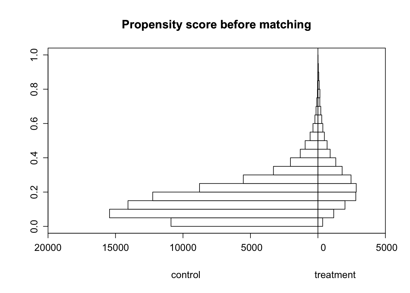
Overlap and its meaning Overlap refers to the degree of similarity or commonality between the treatment group (those who received the treatment being studied) and the control group (those who did not receive the treatment). The overlap is important because it is a necessary condition for the ignorability assumption to hold. If there is no overlap, then the treatment and control groups are so different that it is impossible to make causal inferences. The histogram above shows that there is a only some overlap between the treatment and control group, more individuals in the control group with lower propensity scores than in the treatment group. This is a violation of the Common Support assumption.
Based on the analysis done so far. So, to resolve that I can select only those subjects that can create similarity in the samples.
That will involve following steps:
-Calculate propensity score and match based on propensity values, then rerun all analysis as before. Propensity score calculates the probability that a unit will fall into treatment group.
**Okay: lets begin the real analysis on unbiased data: The steps are:
match the population and rerun ATE
rerun average treatment effect on treated only
perform more analysis matching samples by neighbour method, inverse weighted method
STEP 1. Matching the population with propensity score
Match treated/control mothers using your estimated propensity scores and nearest neighbor matching. Compare the balancing of pretreatment characteristics (covariates) between treated and non-treated units in the original dataset.
## Nearest-neighbor Matching
prospensity_score_matched <- MatchIt::matchit(tobacco ~  mage +  meduc +
                             mblack + alcohol + first + diabete + anemia + birthwgt, data = smoking_data, method = "nearest")

## Covariate Imbalance post matching
matched_prospensity_dataset <- match.data(prospensity_score_matched)

# Drawing back to back histograms for propensity scores for treated and
# non-treated after matching
histbackback(split(matched_prospensity_dataset$prospensity_scores,  matched_prospensity_dataset$tobacco),   main= "Propensity
        score   after   matching",  xlab=c("control",   "treatment"))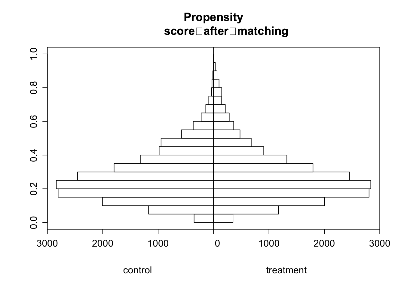
Post matching, there is a better overlap between the treatment and control group. Units with high propensity score is matched with its counterparts and vice versa. This means the units we are comparing between the treatment and control group are similar. This helps us define counterfactuals of what would have happened to the treatment group if they were not treated.
# the covariates between treated and non-treated that were used in the
# estimation of the propensity scores
xBalance(tobacco ~ mage +  meduc + mblack + alcohol + first + diabete + anemia + birthwgt, data = matched_prospensity_dataset,
         report=c("std.diffs","chisquare.test", "p.values"))
strata(): unstrat
stat std.diff
vars
mage 0.0 ***
meduc 0.0 ***
mblack 0.0 **
alcohol 0.1 ***
first 0.0 ***
diabete 0.0 .
anemia 0.0
birthwgt 0.0 *
---Overall Test---
chisquare df p.value
unstrat 175 8 1e-33
---
Signif. codes: 0 '***' 0.001 '** ' 0.01 '* ' 0.05 '. ' 0.1 ' ' 1 xBalance(tobacco ~ mage + meduc + mblack + alcohol + first + diabete + anemia + birthwgt, data = smoking_data,
report=c("std.diffs","chisquare.test", "p.values")) strata(): unstrat
stat std.diff
vars
mage -0.4 ***
meduc -0.6 ***
mblack 0.1 ***
alcohol 0.3 ***
first -0.1 ***
diabete 0.0
anemia 0.1 ***
birthwgt -0.5 ***
---Overall Test---
chisquare df p.value
unstrat 10298 8 0
---
Signif. codes: 0 '***' 0.001 '** ' 0.01 '* ' 0.05 '. ' 0.1 ' ' 1 After the matching, the nature and weight of the regression coefficients changed. Previously in unmatched data, I discussed that with increase age of mother, propensity score decreases. But post matching, the coefficients is showing that propensity score actually increases with increasing age of the mother. This is a sign that matching have accounted fixed effects in the observational dataset. Moreover, some covariates which were significant in determining the treatement status in the pre matching, are not significant anymore post matching. Like diabete, anemia, birthwgt, and mblack. Thus mother being black, having diabetes, and having anaemia, does not determine if she will receive the treatment or not.
But, this conclusion is not yet sufficient. What if I see this change only on treated population and not in control group ? The follwing step involves that:
STEP 2: Average treatment effect on treated group
This step is necessary because it can be more robust estimate. For example: this will compare the change before treatment and after treatment in the same units.
## calculate ATE based on nearest neighbor matching
sumdiff_data <- matched_prospensity_dataset%>%
  group_by(subclass)%>%
  mutate(diff = birthwgt[tobacco==1]- birthwgt[tobacco==0])

dif_in_treated <- sum(sumdiff_data$diff)/2

ATT_weighted_count = 1/sum(matched_prospensity_dataset$tobacco) * dif_in_treated
ATT_weighted_count
[1] -13.361For the treated smoker mothers, the tobacco effects on their child birth weight is lower by 13 grams on average than for its counterfactual non smoking mothers. This means that the treatment has caused lower birth weight in the treated group of mothers. For any other units of population who shares similar covariates as treated group, the birth weight of their child will be lower by 13 grams on average if they were to start smoking tobacco.
Is the conclusion final ? not yet. What if the propensity matching has drawbacks, which it does already. Propensity score matching is based on the fact that all covariates have similar influence in treatment. But, this does not always hold true. WLS matching fixes that.
ATE with WLS Matching
This step is necessary becuase the
## Weighted least Squares (WLS) estimator Preparation
smoking_data <- smoking_data %>%
  mutate(weights = tobacco / prospensity_scores + (1 - tobacco) / (1 - prospensity_scores))

## Weighted least Squares (WLS) Estimates
wls <- lm(birthwgt ~ tobacco + mage +  meduc +
                           mblack + alcohol + first + diabete + anemia,
          data = smoking_data, weights = weights)

summary(wls)
Call:
lm(formula = birthwgt ~ tobacco + mage + meduc + mblack + alcohol +
    first + diabete + anemia, data = smoking_data, weights = weights)

Weighted Residuals:
   Min     1Q Median     3Q    Max
 -7283   -374     32    396  12243

Coefficients:
            Estimate Std. Error t value Pr(>|t|)
(Intercept) 3122.734     11.584  269.58  < 2e-16 ***
tobacco        1.426      3.241    0.44     0.66
mage           0.219      0.358    0.61     0.54
meduc         23.497      0.881   26.69  < 2e-16 ***
mblack      -215.695      4.978  -43.33  < 2e-16 ***
alcohol     -174.499     13.803  -12.64  < 2e-16 ***
first        -65.326      3.509  -18.61  < 2e-16 ***
diabete       72.223     12.213    5.91  3.4e-09 ***
anemia       -23.746     16.766   -1.42     0.16
---
Signif. codes:  0 '***' 0.001 '**' 0.01 '*' 0.05 '.' 0.1 ' ' 1

Residual standard error: 698 on 94163 degrees of freedom
  (1 observation deleted due to missingness)
Multiple R-squared:  0.0369,    Adjusted R-squared:  0.0368
F-statistic:  451 on 8 and 94163 DF,  p-value: <2e-16
## Present resultsThe WLS matching is weighted based on propensity scores, meaning unit with higher similarity in covariates gets more weights. Based on this matching, the average birth weight of children for non smoker mother or control group is 3122.7338, keeping all other variables unchanged. This is statistically significant at 5% signficance. Of all the covariates, mblack covariates has greatest influence in outcome. i.e If the women identifies as black, the birth weight of the child is lower by 241 grams, which is significant. Besides, other covariates like drinking alcohol, first born child, and diabetes in covariates also significantly influence birthweight. However, tobacco appears insignificant at 5 percent signficance level. The model only explains 3 percent of variation given by R squared in birth weight of children. This means that the model is not a good fit for the data.
There are certain factors that influences the output more than other covariates. This was also shown by the coefficients in Balance estimates in previous step. When using ATT with propensity score matching, the model assumed that all covariates has equal influence in determining the treatment status. But in reality, this is not always true. The WLS matching takes weights of each covariates into account, thus providing different output than ATT. if all the covariates had same weights, we would have got same estimate using both ATT and WLS matching.
Is the conclusion final ?
-Statistically YES !