Soccer players attributes comparison: Conclusion from Data visualization
Data Visualization
R
Author
Sujan Bhattarai
Introduction about the project
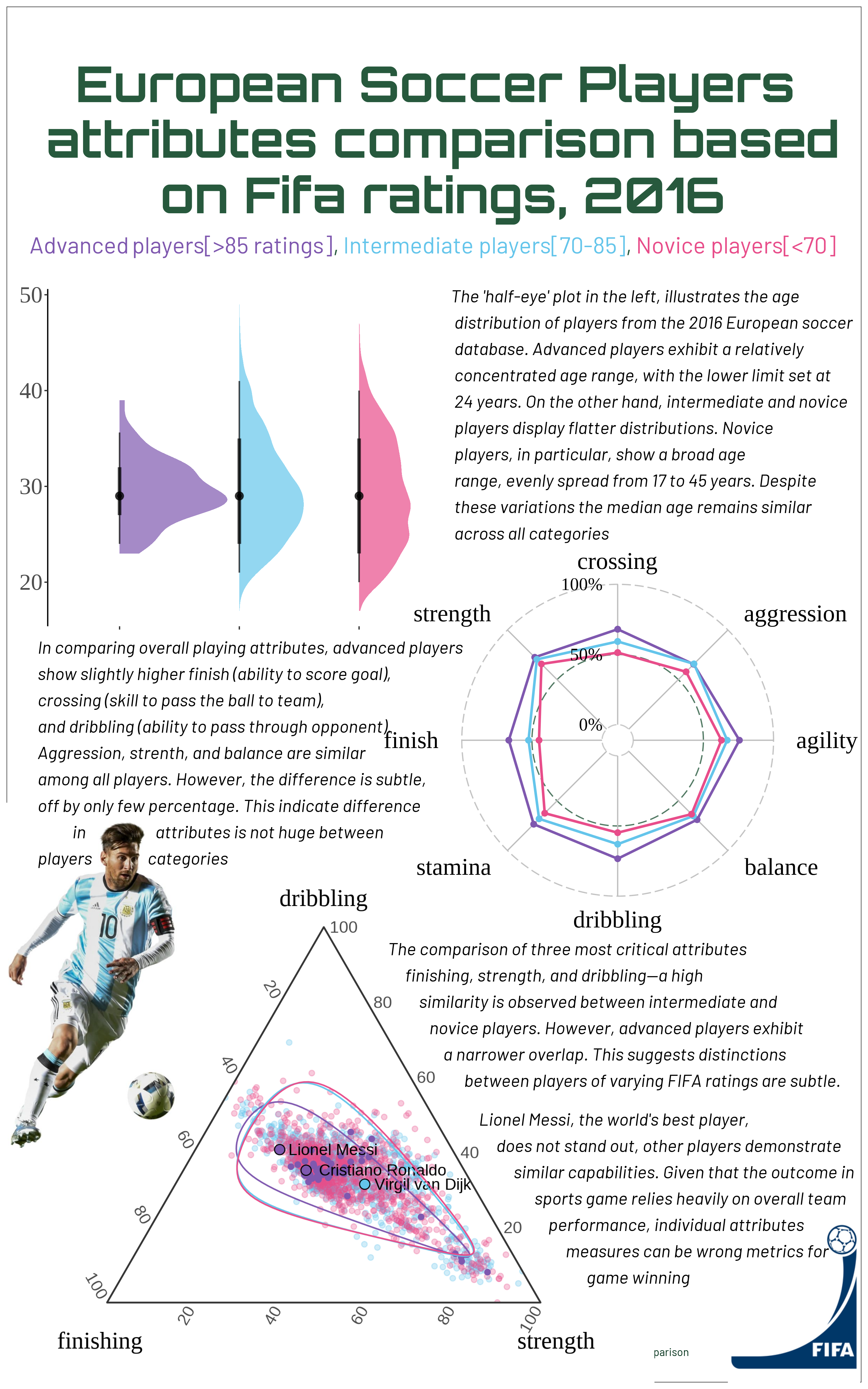
This project aims to create infographics comparing attributes of soccer players, sourced from a European soccer database available on Kaggle. The database contains data on over 10,000 players. Using R exclusively, the visualization focuses on attributes such as shooting, finishing, strength, age, etc. All tasks, from fetching the data to adding text and aligning elements, are performed using R packages. Special credit is given to the UFO alien template, accessible at UFO link
Important Note: The ggplot package version used in this project is 3.4.4, and ggtern version 3.0.0 is utilized. It’s crucial to consider that modern versions of ggplot might conflict when used in combination with other packages employed here.
Data Wrangling
The datasets available on Kaggle are stored in SQLite and require joins to build a complete dataset. However, for this project, data from a single table is sufficient. Nevertheless, for future use, datasets will be combined if necessary.
#read the csv fileplayer_attr <-read_csv(here("featured_projects/data_viz/player_attr.csv"))
The dataset includes a column named “overall ratings,” representing the FIFA average rating from 2008 to 2016. This column will be utilized to categorize players into Advanced, Intermediate, and Novice. It’s important to note that the term “Novice” is used for classification purposes and does not undermine any players; it’s simply a classification based on personal preference.
#---classify the players based on their overall ratingplayer_attr <- player_attr %>%mutate(player_class =ifelse(overall_rating >=85, "Advanced", ifelse(overall_rating >=70& overall_rating <85, "Intermediate", "Novice")))
The project will compare the following attributes of players. The hypothesis is whether there exists a difference in attributes between the world’s renowned top performers and players who do not enjoy the same level of popularity.
# filter required columns from the datasetplayer_data <- player_attr %>%select(player_name, player_class, crossing, agility, dribbling, finishing, aggression, balance, strength, stamina)
From the database containing over 10,000 players, only a subset is required. A random sample of 1000 players will be drawn from the intermediate and novice categories, while all players from the advanced category will be included, given that there are already fewer than 1000 advanced category players.
#---filter only good players from the player_data datasegood_players <- player_data %>%filter(player_class =="Advanced")#---filter average and bad players from the player_data datasetset.seed(123)average_bad_players <- player_data %>%filter(player_class !="Advanced") %>%#sample only 1000 from average and bad playersgroup_by(player_class) %>%#randomly select 1000 players from each class and always include the player Van dijk in the samplesample_n(1000)#good defender van dijkvan_dijk <- player_data %>%filter(player_name =="Virgil van Dijk")#---combine the good_players and average_bad_players datasetsclean_player_data <-bind_rows(good_players, average_bad_players, van_dijk)
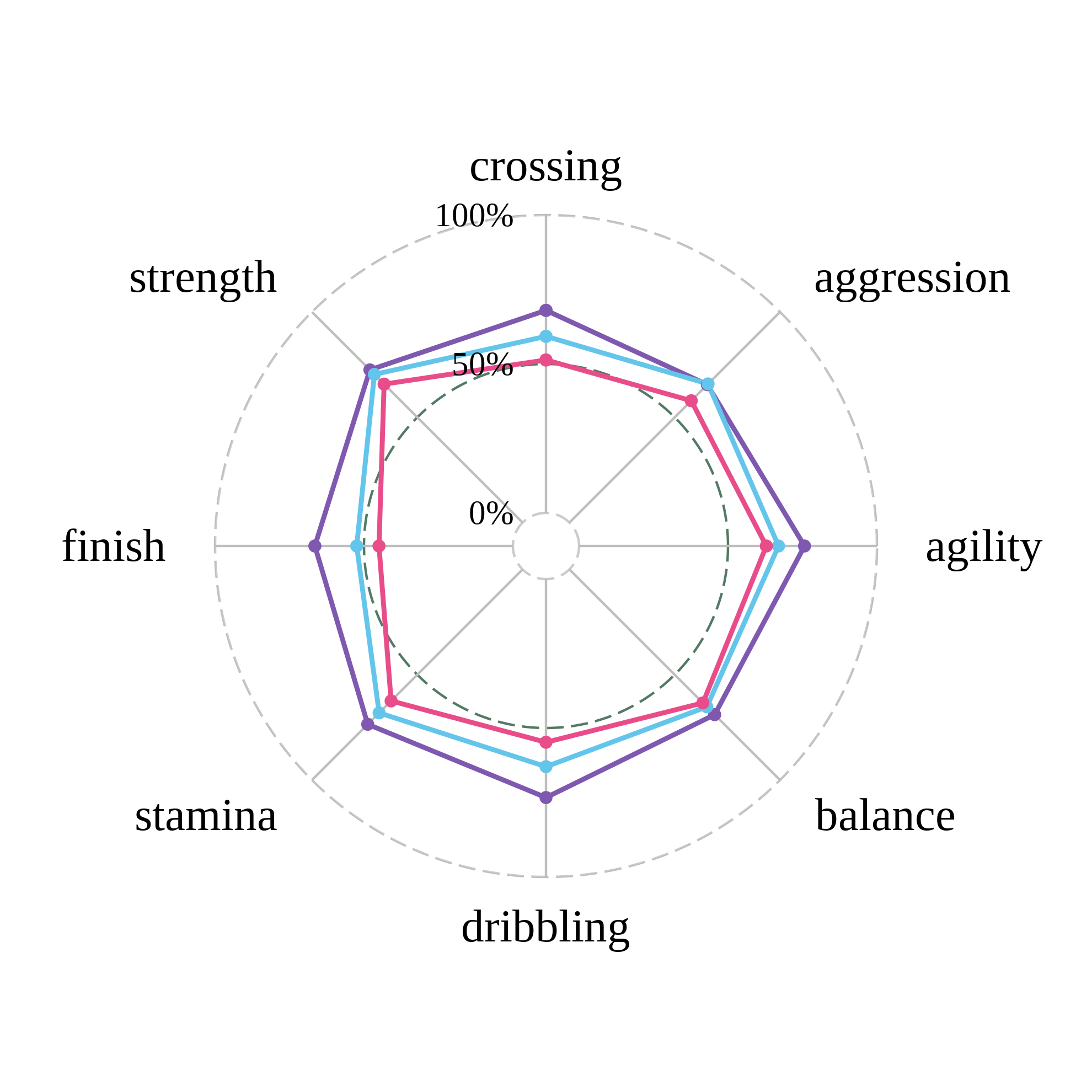
Plot 1: Radar plot for common attributes comparison
#summarize the data and plot the summary output with radar chartradar_data <- clean_player_data %>%group_by(player_class) %>%select(-player_name, player_class) %>%summarise_all(mean, na.rm =TRUE) %>%arrange(ifelse(player_class =="Advanced", 1, ifelse(player_class =="Intermediate", 2, 3))) %>%#arrange so that corssing, finishing, driblling and agility are away from each otherrename("finish"="finishing") %>%select(player_class, crossing, aggression, agility, balance, dribbling, stamina, finish, strength)#create custom color paletteAcolors <-c("#7f58AF", "#64C5EB", "#E84D8A", "#FEB326", "lightblue")radar_plot <- ggradar::ggradar(radar_data,grid.min =0,grid.max =100,grid.mid =50,axis.label.size =22,label.centre.y =FALSE,group.line.width =1,gridline.mid.colour ="#27593d",group.point.size =2,grid.label.size =20,group.colours =c("#7f58AF", "#64C5EB", "#E84D8A"),background.circle.colour ="white",legend.title ="Players proficiency",legend.text.size =24,font.radar ="serif") +#make the background theme whitetheme_void() +#remove y axis labeltheme(axis.text.y =element_blank())+#remove x axis labeltheme(axis.text.x =element_blank())+#remove all grid lines theme(panel.grid.major =element_blank(), panel.grid.minor =element_blank())+#remove legendtheme(legend.position ="none")#save this as pngggsave(plot = radar_plot, filename ="image/radar_plot.png", height =6, width =6, scale =1.1, dpi=300)#Include the radar plot in the rmd#knitr::include_graphics("image/radar_plot.png")knitr::include_graphics("static_image/radar.png")
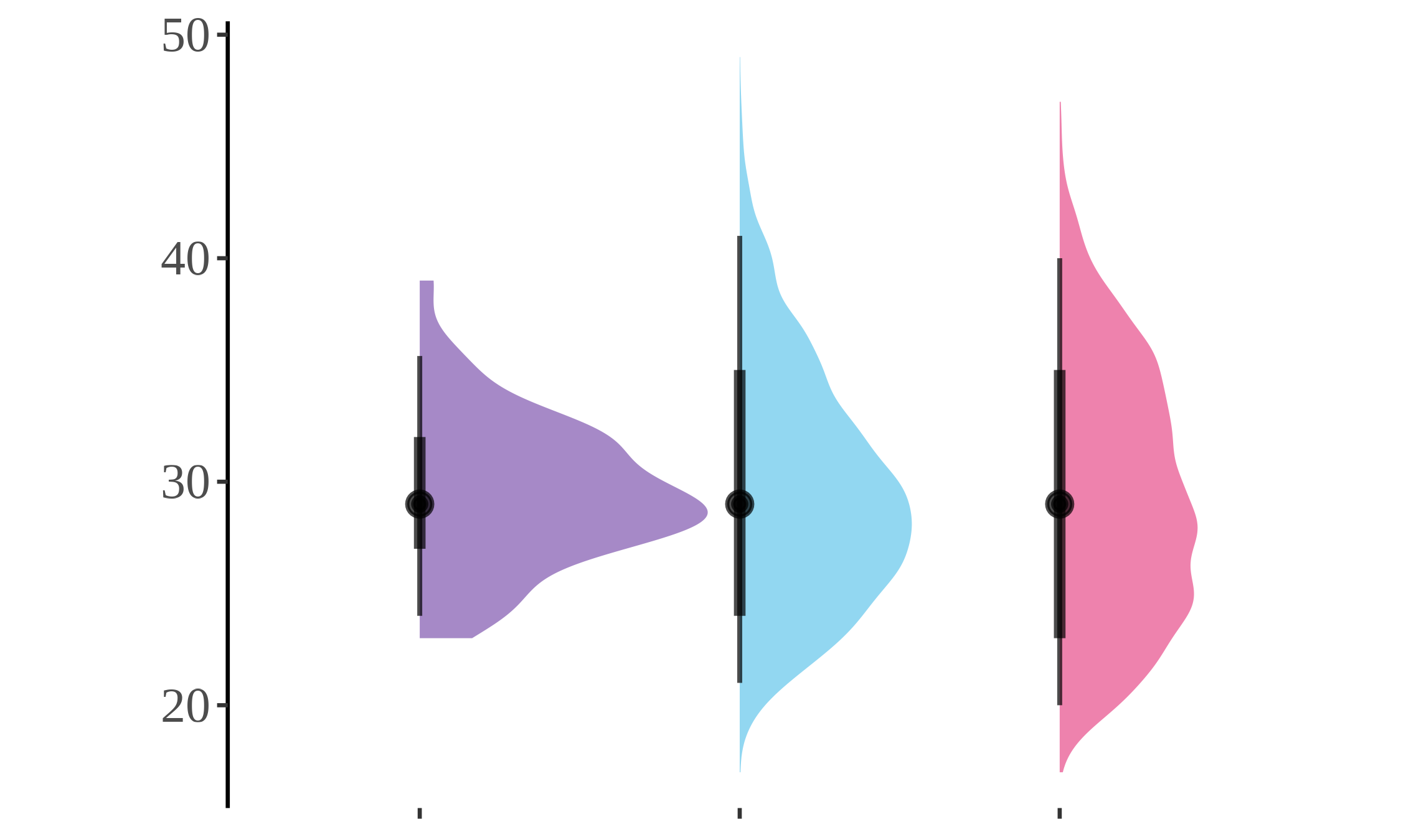
Plot 2: Stat-halfeye plot for age distribution
library(ggdist)##eye plot#plot lefeye plot using stat_halfeyedata <-player_attr %>%mutate(birthday =as.Date(birthday)) %>%mutate(birthday =as.numeric(format(birthday, "%Y"))) %>%#calculate the agemutate(age =2016- birthday)#plot the half eyeeye_plot <-ggplot(data, aes(x = age, y = player_class, fill = player_class))+stat_halfeye(alpha =0.7, color ="black") +theme(panel.background =element_blank(),panel.grid =element_blank(),legend.position ="none",plot.background =element_blank(),panel.border =element_blank(),axis.title.x =element_blank(),axis.line.y =element_line())+theme(legend.position ="none",axis.text =element_text(size =60),axis.title =element_text(size =90),text =element_text(family ="serif"),panel.grid.major =element_blank(),panel.grid.minor =element_blank()) +scale_fill_manual(values = colors) +theme(axis.text.x =element_blank()) +coord_flip() +xlab("") +ylab("")+theme(panel.background =element_blank())#save as ggplotggplot2::ggsave(plot = eye_plot, filename ="image/eye_plot.png", height =3, width =5, dpi =450)#include the age plot in rmd#knitr::include_graphics("image/eye_plot.png")knitr::include_graphics("static_image/eye_plot.png")
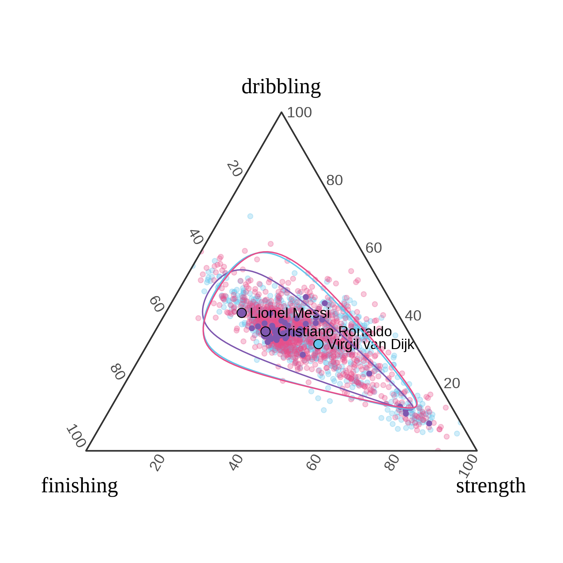
Plot 3: Ternary plot for 3 major attributes comparison
#standarize the clean_player_data for all numeric columns based on min and max valueplayer_standarized <- clean_player_data %>%mutate(across(where(is.numeric), ~scales::rescale(.x, to =c(0, 1))))# Plot the ternary plot for three attributes: strength, aggression, and balance#Plot the ternary plot for three attributes: strength, aggression, and balancetern_plot <- ggtern::ggtern(player_standarized, aes(x = finishing, y = dribbling, z = strength, color = player_class)) +geom_point(alpha =0.3)+theme_bw()+scale_color_manual(values = colors)+# Highlight all points with advanced playersgeom_point(data = player_standarized %>%filter(player_class =="Advanced"), aes(x = finishing, y = dribbling, z = agility))+# Add labels for popular players of presnt datageom_text(data = player_standarized %>%filter(player_name %in%c("Lionel Messi", "Cristiano Ronaldo", "Virgil van Dijk")), aes(label = player_name),alpha =1, hjust =-0.1, hjust =0.5, size =12, color ="black")+# Color the points for Messi and Ronaldogeom_point(data = player_standarized %>%filter(player_name %in%c("Lionel Messi", "Cristiano Ronaldo", "Virgil van Dijk")), aes(x = finishing, y = dribbling, z = strength, fill = player_class), color ='black', shape =21, size =3)+#manual fill color for the highlighted playersscale_fill_manual(values =c("Advanced"="#7f58AF", "Intermediate"="#64C5EB", "Novice"="#E84D8A"))+#remove the legend produced from scale fill manualguides(fill ="none")+#increase axis text sizetheme(axis.text =element_text(size =36))+theme(axis.title =element_text(size =52))+theme(axis.title =element_text(family ="serif"))+#remove the legendtheme(legend.position ="none")+geom_confidence_tern(breaks =0.95)+theme(tern.axis.title.L =element_text(hjust =-.1, vjust =2),tern.axis.title.R =element_text(hjust =1, vjust =2))#save this as jpg using ggsave with name tern_plotggsave(plot = tern_plot, filename ="image/tern_plot.png", height =6 , width =6, dpi =300)#Include the ternary plot in the rmd#knitr::include_graphics("image/tern_plot.png")knitr::include_graphics("static_image/tern_plot.png")
Infographics:aesthetics buildup
This segment and beyond involves, creating text, plots, base plots, etc aesthetics for the final infographics. Most of these are derived from UFO plot, as mentioned in the introduction of this document.
# Define subtitle with HTML formatting for colorssubtitle <-"<span style='color:#7f58AF'>Advanced players[>85 ratings]</span>, <span style='color:#64C5EB'>Intermediate players[70-85]</span>, <span style='color:#E84D8A'>Novice players[<70]</span>"#---------------copy of UFO plotg_base <-ggplot() +labs(title ="European Soccer Players \n attributes comparison based \n on Fifa ratings, 2016",subtitle = subtitle,caption = caption ) +theme_void() +theme(text =element_text(family = ft, size =36, lineheight =0.3, colour = txt),plot.background =element_rect(fill ="white", colour = bg),plot.title =element_text(size =128, face ="bold", hjust =0.5, margin =margin(b =10)),plot.subtitle =element_text(family = ft1, hjust =0.5, margin =margin(b =20), color ="#27593d", size =60),plot.caption =element_markdown(family = ft1, colour = colorspace::darken(txt, 0.5), hjust =0.5,margin =margin(t =20)),plot.margin =margin(b =20, t =50, r =50, l =50),axis.text.x =element_text())+theme(plot.subtitle =element_markdown() )# # quote 1 for the distributionquote1 <-ggplot() +annotate("text", x =0, y =1, label ="The 'half-eye' plot in the left, illustrates the age \n distribution of players from the 2016 European soccer \n database. Advanced players exhibit a relatively \n concentrated age range, with the lower limit set at \n 24 years. On the other hand, intermediate and novice \n players display flatter distributions. Novice \n players, in particular, show a broad age \n range, evenly spread from 17 to 45 years. Despite \n these variations the median age remains similar \n across all categories",family = ft1, colour ='black', size =16, hjust =0, fontface ="italic", lineheight =0.4) +xlim(0, 1) +ylim(0, 1) +theme_void() +coord_cartesian(clip ="off")quote2 <-ggplot() +annotate("text", x =0, y =1, label =" In comparing overall playing attributes, advanced players \n show slightly higher finish (ability to score goal),\n crossing (skill to pass the ball to team), \n and dribbling (ability to pass through opponent).\n Aggression, strenth, and balance are similar \n among all players. However, the difference is subtle,\n off by only few percentage",family = ft1, colour ='black', size =16, hjust =0, fontface ="italic", lineheight =0.4) +xlim(0, 1) +ylim(0, 1) +theme_void() +coord_cartesian(clip ="off")#quote 3quote3 <-ggplot() +annotate("text", x =0, y =1, label ="The comparison of three most critical attributes \n finishing, strength, and dribbling—a high \n similarity is observed between intermediate and \n novice players. However, advanced players exhibit \n a narrower overlap. This suggests distinctions \n between players of varying FIFA ratings are subtle.",family = ft1, colour ='black', size =16, hjust =0, fontface ="italic", lineheight =0.4) +xlim(0, 1) +ylim(0, 1) +theme_void() +coord_cartesian(clip ="off")quote4 <-ggplot()+annotate("text", x=0, y =1, label ="Lionel Messi, the world's best player,\n does not stand out, other players demonstrate \n similar capabilities. Given that the outcome in \n sports game relies heavily on overall team \n performance, individual attributes \n measures can be wrong metrics for\n game winning",family = ft1, colour ="black", size =16, hjust =0, fontface ="italic", lineheight =0.4) +xlim(0, 1) +ylim(0, 1) +theme_void() +coord_cartesian(clip ="off")
Images cannot be loaded into ggplot object directly. it should be convereted to raster object and then it can be overlaid over other ggplot object. The following codes achieves the same thing for different images that are used in the final infographics.
#load the tern imageimage <-readPNG("image/tern_plot.png")tern_image <-as.raster(image)#radar plotradar <-readPNG("image/radar_plot.png")radar_image <-as.raster(radar)#tern plot imageimage <-readPNG("image/tern_plot.png")image <-as.raster(image)#lionel messi imagemessi <-readJPEG("data/images/messi.jpg")messi <-as.raster(messi)#fifa logo imagefifa <-readPNG("data/images/FIFA.png")fifa <-as.raster(fifa)#goalpost as imagesoccer_field <-readJPEG("data/images/soccer-field.jpg")soccer_field <-as.raster(soccer_field)
The final graph is produced from the following line. This chunk adds all previously made plots and inset them into appropriate locations, based on preference. This process takes really long time, as finding the exact location from just point values is significantly tedious task. I would suggest using any other graphical interface software to add the quotes and paragraphs, which takes way less time.
# Combine the plots into a single infographicg_final <- g_base +inset_element(fifa, left =0.9, right =1.08, top =0.25, bottom =-0.2)+inset_element(eye_plot, left =-0.12, right =0.57, top =1, bottom =0.66) +#insert radar plotinset_element(tern_image, left =-0.10, right =0.80, top =0.5, bottom =-.1) +inset_element(messi, left =-0.08, right =0.15, top =0.50, bottom =0.15) +inset_element(radar_plot, left =0.4, right =1.1, top =0.81, bottom =0.31) +#insert quote 1inset_element(quote1, left =0.5, right =1, top =0.88, bottom =0.72) +#Insert quote 2inset_element(quote2, left =-0.07, right =0.5, top =0.55, bottom =0.5) +#insert quote 3inset_element(quote3, left =0.41, right =1, top =0.31, bottom =0) +#insert quote 4inset_element(quote4, left =0.54, right =1, top =0.13, bottom =-0.10)+plot_annotation(theme =theme(plot.background =element_rect(fill ="white", colour ='white')))ggsave(plot = g_final, filename ="infographics_draft.png", height =16, width =10)