Using AI for Good: Helping non profits in predicting carbon calculation

Technologies: Machine Learning, Python, XGBoost, Linear Regression
Author: Sujan Bhattarai

Project Overview

This project supports a marine research organization (established in 1910) in developing predictive models for ocean carbon concentrations—a critical component of marine ecosystem health. The organization’s extensive time series dataset provides invaluable insights into environmental changes affecting Pacific marine ecosystems and the communities that depend on them.

Objective

Develop accurate machine learning models to predict dissolved inorganic carbon (DIC) concentrations in ocean waters using various oceanographic parameters. These predictions will enhance understanding of marine carbon cycles and support data-driven conservation decisions.

Dataset Description

• Size: 12 columns with 1 target variable and 11 predictors
• Target Variable: Dissolved Inorganic Carbon (DIC) concentration
• Features: Physical and chemical ocean properties including temperature, salinity, oxygen concentration, and geographical coordinates
• Scope: California Current System extending to North Pacific waters

Methodology

1. Data Preprocessing and Exploration

• Standardized column naming conventions
• Removed columns with missing or inappropriate values
• Applied correlation analysis to understand feature relationships
• Visualized data patterns using correlation heatmaps

2. Model Development

Linear Regression with Polynomial Features

• Approach: Implemented polynomial feature engineering with regularization
• Optimization: Tested polynomial degrees (1-5) and Ridge regularization parameters
• Pipeline: PolynomialFeatures → StandardScaler → Ridge Regression
• Best Configuration: Degree 1 polynomial with alpha=50 regularization

XGBoost Implementation

• Base Model: Out-of-the-box XGBoost with cross-validation
• Hyperparameter Tuning: Grid search optimization across multiple parameters
• Final Parameters:
  • n_estimators: 1450
  • max_depth: 5
  • learning_rate: 0.01
  • colsample_bytree: 0.5

3. Model Evaluation and Validation

• Applied train-validation-test splits for robust evaluation
• Used cross-validation with early stopping to prevent overfitting
• Compared models using R² scores and RMSE metrics

Key Results

Model	Training R²	Validation R²	RMSE
Linear Regression	0.9964	0.9964	~6.0
XGBoost	0.9979	0.9979	3.61

Key Findings

1. Strong Predictive Performance: Both models achieved high accuracy (>99.6% R²), indicating robust relationships between oceanographic parameters and carbon concentrations.

2. XGBoost Superiority: The gradient boosting model outperformed linear regression with:

   • Higher validation accuracy (0.9979 vs 0.9964)
   • Lower prediction error (RMSE: 3.61 vs ~6.0)
   • Better handling of complex feature interactions

3. Feature Importance: Physical and chemical ocean properties demonstrate strong predictive power for carbon concentration levels.

Technical Implementation

# Key libraries and frameworks used
- scikit-learn: Model development and evaluation
- XGBoost: Gradient boosting implementation
- pandas/numpy: Data manipulation and analysis
- matplotlib/seaborn: Data visualization
- GridSearchCV: Hyperparameter optimization

::: {.cell}

```{.python .cell-code}
#hide all warnings
import warnings
warnings.filterwarnings("ignore")

#### Import all necessary libraries
# import all required libraries
import numpy as np
import xgboost as xgb
import pandas as pd
import seaborn as sns
import matplotlib as mpl
import matplotlib.pyplot as plt
from sklearn.model_selection import train_test_split
from sklearn.pipeline import make_pipeline
from sklearn.preprocessing import StandardScaler
from sklearn.model_selection import GridSearchCV
from sklearn.linear_model import LinearRegression
from sklearn.metrics import mean_squared_error
from sklearn.model_selection import cross_val_score, KFold
from sklearn.linear_model import SGDRegressor
from sklearn.linear_model import Ridge
from sklearn.preprocessing import PolynomialFeatures

:::

Read the data and store ID:required during submission for validity check

#-----read train and test set
train_calcofi = pd.read_csv("data/train.csv")
test_calcofi  = pd.read_csv("data/test.csv")  

#collect the test ids for testcalcofi, required for submission dataset
test_ids = test_calcofi.id
test_calcofi = test_calcofi.drop(columns=['id'])

Data cleaning

A model is only as good as the data.This step ensures that columns names are standarized, and the columns with inappropriate values are removed. The data is also checked for missing values. Incase of missing values, they are not imputed, but dropped. The CALCOFI did not provide claer guidance on how value should be imputted. So the best decision is to drop the rows with missing values.

#----inspect the head and take the insights of data
train_calcofi.head()

   id    Lat_Dec     Lon_Dec  ...  Salinity1  Temperature_degC      DIC
0   1  34.385030 -120.665530  ...     34.198              7.82  2270.17
1   2  31.418333 -121.998333  ...     34.074              7.15  2254.10
2   3  34.385030 -120.665530  ...     33.537             11.68  2111.04
3   4  33.482580 -122.533070  ...     34.048              8.36  2223.41
4   5  31.414320 -121.997670  ...     34.117              7.57  2252.62

[5 rows x 19 columns]

#### Data cleaning and preprocessing
#the column names are in snake case, change all to lowercase
train_calcofi.columns = map(str.lower, train_calcofi.columns)
test_calcofi.columns = map(str.lower, test_calcofi.columns)

#remove the unnamed:12 column
train_calcofi = train_calcofi.drop(columns=['unnamed: 12'])
train_calcofi.rename(columns={'ta1.x': 'ta1'}, inplace=True)

The data looks clean. Now, a relationships between columns must be established This helps in understanding the data, and also helps in feature selection. The next step below plots a correlation matrix. This will show correlated variables in the dataset.

The reason that the correlation matrix is plotted to see if linear regression can be useful. If the correlation matrix shows strong relationship between the response and predictors, then linear regression is a great algorithm. If not, then other models must be tested.

#plot correlation matrix
corr_matrix = train_calcofi.corr()

# Plot the heatmap
plt.figure(figsize=(8, 6))
sns.heatmap(corr_matrix, annot=False, cmap='coolwarm', fmt=".1f")
plt.title('Correlation Heatmap')
plt.show()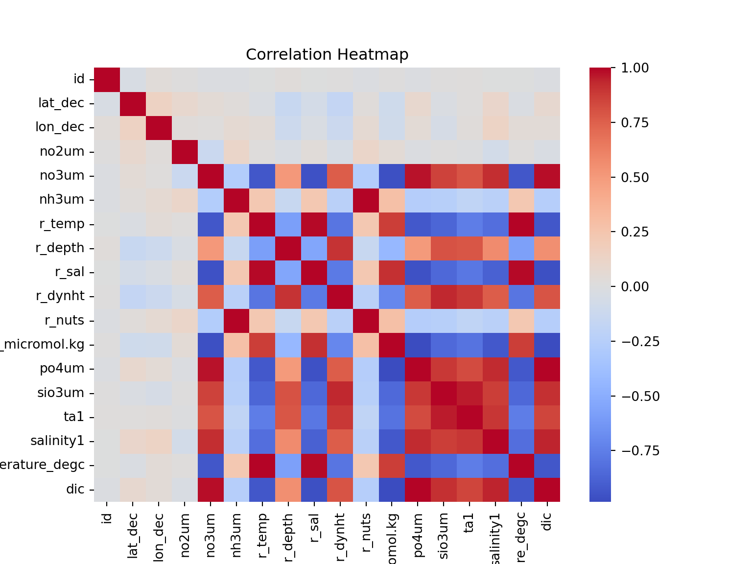

Linear regression model

# Select only the predictors columns, and change them to array
X = train_calcofi.drop(columns=['dic', 'id'], axis=1)

# Select only the response column and change it to array
y = train_calcofi['dic']

# Split the data into training, validation, and test sets
X_train, X_temp, y_train, y_temp = train_test_split(X, y, test_size=0.4, random_state=42)
X_val, X_test, y_val, y_test = train_test_split(X_temp, y_temp, test_size=0.5, random_state=42)

# Define the range of polynomial degrees to fit
degrees = range(1, 5)  # From 1 to 5

# Initialize lists to store R^2 scores
train_r2_scores = []
val_r2_scores = []

# Loop through each polynomial degree
for degree in degrees:
    # Create a pipeline with PolynomialFeatures, StandardScaler, and LinearRegression
    model_pipeline = make_pipeline(PolynomialFeatures(degree=degree), StandardScaler(), LinearRegression())

    # Fit the model pipeline to the training data
    model_pipeline.fit(X_train, y_train)

    # Calculate R^2 on the training set
    train_r2 = model_pipeline.score(X_train, y_train)
    train_r2_scores.append(train_r2)

    # Calculate R^2 on the validation set
    val_r2 = model_pipeline.score(X_val, y_val)
    val_r2_scores.append(val_r2)

    # Print the results for each degree
    print(f"Degree: {degree}")
    print(f"  R^2 on training set: {train_r2}")
    print(f"  R^2 on validation set: {val_r2}")
    print("-" * 40)

Pipeline(steps=[('polynomialfeatures', PolynomialFeatures(degree=4)),
                ('standardscaler', StandardScaler()),
                ('linearregression', LinearRegression())])

In a Jupyter environment, please rerun this cell to show the HTML representation or trust the notebook.
On GitHub, the HTML representation is unable to render, please try loading this page with nbviewer.org.

# Plotting the R^2 scores for training and validation sets
plt.figure(figsize=(10, 6))
plt.plot(degrees, train_r2_scores, label='Training R^2', marker='o')
plt.plot(degrees, val_r2_scores, label='Validation R^2', marker='o')
plt.xlabel('Polynomial Degree')
plt.ylabel('R^2 Score')
plt.title('Polynomial Degree vs. R^2 Score')
plt.legend()
plt.grid(True)
plt.show()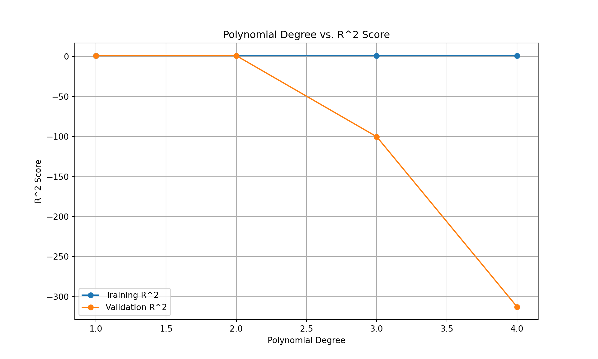

#from the above sample, it is clear that either degree 1 or 2 is best
# Define the polynomial degree
degree = 1

# Define the range of regularization parameters (alpha values) to test
alphas = np.logspace(-3, 3,  10)  # e.g., 10^-4 to 10^4

# Initialize lists to store R^2 scores
train_r2_scores = []
val_r2_scores = []

# Loop through each alpha value
for alpha in alphas:
    # Create a pipeline with PolynomialFeatures, StandardScaler, and Ridge regression
    model_pipeline = make_pipeline(PolynomialFeatures(degree=degree), StandardScaler(), Ridge(alpha=alpha))

    # Fit the model pipeline to the training data
    model_pipeline.fit(X_train, y_train)

    # Calculate R^2 on the training set
    train_r2 = model_pipeline.score(X_train, y_train)
    train_r2_scores.append(train_r2)

    # Calculate R^2 on the validation set
    val_r2 = model_pipeline.score(X_val, y_val)
    val_r2_scores.append(val_r2)

    # Print the results for each alpha
    print(f"Alpha: {alpha}")
    print(f"  R^2 on training set: {train_r2}")
    print(f"  R^2 on validation set: {val_r2}")
    print("-" * 40)

Pipeline(steps=[('polynomialfeatures', PolynomialFeatures(degree=1)),
                ('standardscaler', StandardScaler()),
                ('ridge', Ridge(alpha=np.float64(1000.0)))])

In a Jupyter environment, please rerun this cell to show the HTML representation or trust the notebook.
On GitHub, the HTML representation is unable to render, please try loading this page with nbviewer.org.

# Plotting the R^2 scores for training and validation sets
plt.figure(figsize=(12, 6))
plt.plot(alphas, train_r2_scores, label='Training R^2', marker='o', linestyle='-', color='b')
plt.plot(alphas, val_r2_scores, label='Validation R^2', marker='o', linestyle='-', color='r')
plt.xscale('log')  # Log scale for alpha values
plt.xlabel('Regularization Parameter (Alpha)')
plt.ylabel('R^2 Score')
plt.title('Regularization Parameter (Alpha) vs. R^2 Score')
plt.legend()
plt.grid(True)
plt.show()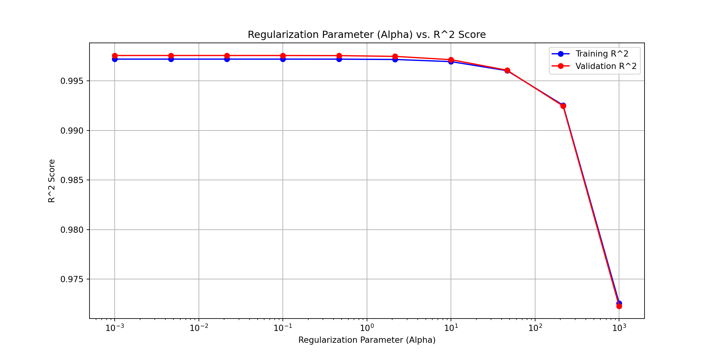

#finalize the model
# Split data into training and validation sets
X_train, X_val, y_train, y_val = train_test_split(X, y, test_size=0.2, random_state=42)

# Define the polynomial degree and regularization parameter (lambda)
degree = 1
alpha = 50  # Regularization parameter

# Create and fit the model pipeline
model_pipeline = make_pipeline(
    PolynomialFeatures(degree=degree),
    StandardScaler(),
    Ridge(alpha=alpha)
)

# Fit the model to the training data
model_pipeline.fit(X_train, y_train)

Pipeline(steps=[('polynomialfeatures', PolynomialFeatures(degree=1)),
                ('standardscaler', StandardScaler()),
                ('ridge', Ridge(alpha=50))])

In a Jupyter environment, please rerun this cell to show the HTML representation or trust the notebook.
On GitHub, the HTML representation is unable to render, please try loading this page with nbviewer.org.

# Evaluate the model
train_r2 = model_pipeline.score(X_train, y_train)
val_r2 = model_pipeline.score(X_val, y_val)

print(f"Training R^2 score for Linear regression: {train_r2}")

Training R^2 score for Linear regression: 0.9964417610035372

print(f"Validation R^2 score for linear regression: {val_r2}")

Validation R^2 score for linear regression: 0.9964454374974873

The base linear regression model has worked well with 1 degree polynomial and low regularization parameters, with mean squared error of 36 on testing set, meaning ocean carbon values(DIC) was off by 36 point on average for the prediction test.

Can XGBoost perform better ?

The next step involves using XGboost for making the prediction, Extreme Gradient Boosting, also called the queen of the ML models is one of the most robust models. Base XGBOOST model (no tuning: Out of Box model) Note:XGBoost works on its own object type, which is Dmatrix. So, datatype conversion is required.

# Create regression matrices, this is requirement for xgboost model
dtrain_reg = xgb.DMatrix(X_train, y_train, enable_categorical=True)
dtest_reg =  xgb.DMatrix(X_test, y_test, enable_categorical=True)

# use cross validation approach to catch the best boosting round
n = 1000

model_xgb = xgb.cv(
   dtrain=dtrain_reg,
   params = {},
   num_boost_round= n,
   nfold = 20, #number of folds for cross validation
   verbose_eval=10, #record rmse every 10 interval
   early_stopping_rounds = 5,
   as_pandas = True#stop if there is no improvement in 5 consecutive rounds
)

[0] train-rmse:79.31111+0.22480 test-rmse:79.31059+4.50293
[10]    train-rmse:4.32181+0.05969  test-rmse:6.83483+2.17431
[20]    train-rmse:2.11548+0.06541  test-rmse:6.12915+2.26123
[30]    train-rmse:1.64633+0.06258  test-rmse:6.04879+2.23034
[40]    train-rmse:1.29777+0.05879  test-rmse:6.02162+2.23979
[50]    train-rmse:1.02154+0.05521  test-rmse:5.99733+2.23518
[54]    train-rmse:0.93376+0.05252  test-rmse:6.00336+2.23321

# Extract the optimal number of boosting rounds
optimal_boosting_rounds = model_xgb['test-rmse-mean'].idxmin()

# #using validation sets during training
evals = [(dtrain_reg, "train"), (dtest_reg, "validation")]

model_xgb = xgb.train(
   params={},
   dtrain=dtrain_reg,
   num_boost_round= optimal_boosting_rounds,
   evals=evals,#print rmse for every iterations
   verbose_eval=10, #record rmse every 10 interval
   early_stopping_rounds = 5 #stop if there is no improvement in 5 consecutive rounds
)

[0] train-rmse:79.30237 validation-rmse:79.79093
[10]    train-rmse:4.39108  validation-rmse:4.91840
[20]    train-rmse:2.09378  validation-rmse:3.83489
[30]    train-rmse:1.63902  validation-rmse:3.79141
[40]    train-rmse:1.30465  validation-rmse:3.68415
[48]    train-rmse:1.08249  validation-rmse:3.61313

# #predict on the the test matrix
preds = model_xgb.predict(dtest_reg)

#check for rmse
# Predict and calculate RMSE manually (fix for older sklearn)
mse = mean_squared_error(y_test, preds)
rmse = np.sqrt(mse)
print(f"RMSE of the test model: {rmse:.3f}")

RMSE of the test model: 3.613

**GRID TUNED XGBOOST MODEL

# Define the parameter grid
gbm_param_grid = {
    'colsample_bytree': [0.5, 0.7, 0.9],
    'n_estimators': [100, 200, 300, 1450],
    'max_depth': [5, 7, 9],
    'learning_rate': [0.001, 0.01]
}

#best hyperparameters based on running
gbm_param_grid_set = {
    'colsample_bytree': [0.5],
    'n_estimators': [1450],
    'max_depth': [5],
    'learning_rate': [0.01]
}

# Instantiate the regressor
gbm = xgb.XGBRegressor()

# Instantiate GridSearchCV with seed
gridsearch_mse = GridSearchCV(
    param_grid=gbm_param_grid_set,
    estimator=gbm,
    scoring='neg_mean_squared_error',
    cv=10,
    verbose=1,
)

# Fit the gridmse
gridsearch_mse.fit(X_train, y_train)

GridSearchCV(cv=10,
             estimator=XGBRegressor(base_score=None, booster=None,
                                    callbacks=None, colsample_bylevel=None,
                                    colsample_bynode=None,
                                    colsample_bytree=None, device=None,
                                    early_stopping_rounds=None,
                                    enable_categorical=False, eval_metric=None,
                                    feature_types=None, gamma=None,
                                    grow_policy=None, importance_type=None,
                                    interaction_constraints=None,
                                    learning_rate=None,...
                                    max_cat_to_onehot=None, max_delta_step=None,
                                    max_depth=None, max_leaves=None,
                                    min_child_weight=None, missing=nan,
                                    monotone_constraints=None,
                                    multi_strategy=None, n_estimators=None,
                                    n_jobs=None, num_parallel_tree=None,
                                    random_state=None, ...),
             param_grid={'colsample_bytree': [0.5], 'learning_rate': [0.01],
                         'max_depth': [5], 'n_estimators': [1450]},
             scoring='neg_mean_squared_error', verbose=1)

In a Jupyter environment, please rerun this cell to show the HTML representation or trust the notebook.
On GitHub, the HTML representation is unable to render, please try loading this page with nbviewer.org.

# Best estimator
best_estimator = gridsearch_mse.best_estimator_

# Use the best estimator to make predictions on the test data
y_pred = best_estimator.predict(X_test)

# Calculate mean squared error
mse_xgboost = mean_squared_error(y_test, y_pred)
print("Training Mean Squared Error:", mse_xgboost)

Training Mean Squared Error: 8.67761675628923

# Now, use the best estimator to make predictions on the validation data
y_val_pred = best_estimator.predict(X_val)

# Calculate mean squared error on the validation set
mse_xgboost_val = mean_squared_error(y_val, y_val_pred)
print("Validation Mean Squared Error:", mse_xgboost_val)

Validation Mean Squared Error: 28.547789322680313

# Get the model score on the validation set
print(f"Model score on validation set: {best_estimator.score(X_val, y_val)}")

Model score on validation set: 0.9978644010412603

print(f"Model score on validation setfor linear regression: {val_r2}")

Model score on validation setfor linear regression: 0.9964454374974873

print(f"Model score on validation set for XGBoost: {best_estimator.score(X_val, y_val)}")

Model score on validation set for XGBoost: 0.9978644010412603

The XGBoost model has lower Bias, and high accuracy compared to the linear regression model. Thus, I suggest using the XGBOOST model for any new incoming data on ocean values.